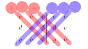
∣∣∣∣∣∣∣adgbehcfi∣∣∣∣∣∣∣=aei−afh−bdi+bfg+cdh−ceg
Determinants of 3x3 matrices can be determined in two ways: Cofactor Method and Basket Weaving Method
Cofactor Method
Choose a row or column (henceforth referred to as N)
Find the minor of each element in N
Multiply each element by its respective minor and add or subtract based on this pattern ⎣⎢⎡+−+−+−+−+⎦⎥⎤
Example 1.1 & 1.2
Evaluate ∣∣∣∣∣∣∣−14−72583−69∣∣∣∣∣∣∣ using the cofactor method.
Example 1.1 Using top row ∣∣∣∣∣∣∣−14−72583−69∣∣∣∣∣∣∣
1. Elements are −1, 2, 3
2. Calculate minors 2a. Minor for −1 is ∣∣∣∣∣58−69∣∣∣∣∣=(5)(9)−(−6)(8)=93 2b. Minor for 2 is ∣∣∣∣∣4−7−69∣∣∣∣∣=(4)(9)−(−6)(−7)=−6 2c. Minor for 3 is ∣∣∣∣∣4−758∣∣∣∣∣=(4)(8)−(5)(−7)=67
3. (−1)(93)−(2)(−6)+(3)(67)=120Example 1.2 Using middle column ∣∣∣∣∣∣∣−14−72583−69∣∣∣∣∣∣∣
1. Elements are 2, 5, 8
2. Calculate minors 2a. Minor for 2 is ∣∣∣∣∣4−7−69∣∣∣∣∣=(4)(9)−(−6)(−7)=−6 2b. Minor for 5 is ∣∣∣∣∣−1−739∣∣∣∣∣=(−1)(9)−(3)(−7)=12 2c. Minor for 8 is ∣∣∣∣∣−143−6∣∣∣∣∣=(−1)(−6)−(3)(4)=−6
3. −(2)(−6)+(5)(12)−(8)(−6)=120
Basket Weaving Method
Copy the first two columns to the right of the matrix
Multiply the elements in each diagonal as shown in the image
Add the ones going down, subtract the ones going up
Example 1.3
Evaluate ∣∣∣∣∣∣∣−14−72583−69∣∣∣∣∣∣∣ using the basket-weaving method
The first three are added and the last three are subtracted
(−45+84+96)−(−105+48+72)=120
Cramer's Rule
Method of solving a system of 3 linear equations of 3 variables
The system of equations a1x+b1y+c1z=C1a2x+b2y+c2z=C2a3x+b3y+c3z=C3
can be represented in matrix form as ⎣⎢⎡a1a2a3b1b2b3c2c2c3⎦⎥⎤⎣⎢⎡xyz⎦⎥⎤=⎣⎢⎡C1C2C3⎦⎥⎤
and the solutions are x=∣∣∣∣∣∣∣a1a2a3b1b2b3c2c2c3∣∣∣∣∣∣∣∣∣∣∣∣∣∣C1C2C3b1b2b3c1c2c3∣∣∣∣∣∣∣,y=∣∣∣∣∣∣∣a1a2a3b1b2b3c2c2c3∣∣∣∣∣∣∣∣∣∣∣∣∣∣a1a2a3C1C2C3c1c2c3∣∣∣∣∣∣∣,z=∣∣∣∣∣∣∣a1a2a3b1b2b3c2c2c3∣∣∣∣∣∣∣∣∣∣∣∣∣∣a1a2a3b1b2b3C1C2C3∣∣∣∣∣∣∣
Example 1.4
Solve the following system using Cramer's Rule −12x−4y+4z=−210x+0y−4z=612x+12y+4z=−1
The matrix form is ⎣⎢⎡−12012−40124−44⎦⎥⎤⎣⎢⎡xyz⎦⎥⎤=⎣⎢⎡−216−1⎦⎥⎤
The denominator is the determinant of the 3x3 matrix
This is easily computed using cofactor method on the second row, taking advantage of the 0s ∣∣∣∣∣∣∣−12012−40124−44∣∣∣∣∣∣∣=−0+0−(−4){(−12)(12)−(−4)(12)}=−384
Finally, we can use the formula for each variable
Start with x, using cofactor method on the second row x=−384∣∣∣∣∣∣∣−216−1−40124−44∣∣∣∣∣∣∣=−384−6{(−4)(4)−(4)(12)}+0−(−4){(−21)(12)−(−4)(−1)}=−384384−1024=35
Next y, using cofactor method on the second row y=−384∣∣∣∣∣∣∣−12012−216−14−44∣∣∣∣∣∣∣=−384−0+6{(−12)(4)−(4)(12)}−(−4){(−12)(−1)−(−21)(12)}=−384−0+(−576)−(−1056)=−45
Finally z, using cofactor method on the second row z=−384∣∣∣∣∣∣∣−12012−4012−216−1∣∣∣∣∣∣∣=−384−0+0−6{(−12)(12)−(−4)(12)}=−384−0+0−(−576)=−23
So the solution to the system is (x,y,z)=(35,−45,−23)
Inverse Matrix
The inverse of matrix M is M−1, and satisfies M−1M=I, where I is the identity matrix M−1 exists if and only ifdetM=0
If M−1 does not exist, the matrix is singular
The inverse matrix can be found in three ways: from the Adjugate Matrix, Gauss-Jordan Elimination/Row Reduction, or with a calculator
Adjugate Matrix
Transpose the matrix (reflect each element across the main diagonal) (MT)
Find the 2x2 minor of each element
Create a 3x3 matrix from the minors, changing signs based on the pattern ⎣⎢⎡+−+−+−+−+⎦⎥⎤
If you have an n×n matrix, append the n×n identity matrix to the right.
The goal is to use the following 3 rules to turn the original matrix into the identity matrix.
This will make the identity matrix turn into the inverse matrix.
Rules
Multiply a row by a non-zero constant
Add a non-zero multiple of one row to another
Swap rows
Example 1.6: 2x2 Matrix
Find the inverse of [2135] using Row Reduction
Append the identity matrix. The divider is added to differentiate the two matrices. [2135∣∣1001]
Swap the two rows to get a 1 in the top left. [1253∣∣0110]
Add −2 times the top row and add it to the bottom row [12−2(1)53−2(5)∣∣01−2(0)10−2(1)]=[105−7∣∣011−2]
Multiply the bottom row by −71 to get the bottom row to be 01 [1−705−7−7∣∣0−711−7−2]=[1051∣∣0−71172]
Finally subtract 5 times the bottom row from the top row to remove the 5 [1−5(0)05−5(1)1∣∣0−5(−71)−711−5(72)72]=[1001∣∣75−71−7372]
So [2135]−1=[75−71−7372]
Example 1.7: 3x3 Matrix
Find the inverse of ⎣⎢⎡44−3−41−34−2−4⎦⎥⎤
Append the identity matrix. The divider is added to differentiate the two matrices. ⎣⎢⎡44−3−41−34−2−4∣∣∣100010001⎦⎥⎤
Multiply the top row by 41 ⎣⎢⎡444−34−41−344−2−4∣∣∣4100010001⎦⎥⎤=⎣⎢⎡14−3−11−31−2−4∣∣∣4100010001⎦⎥⎤
Subtract 4 times the top row from the middle row and add 3 times the top row from the bottom row ⎣⎢⎡14−4(1)−3+3(1)−11−4(−1)−3+3(−1)1−2−4(1)−4+3(1)∣∣∣410−4(41)0+3(41)01−4(0)0+3(0)00−4(0)1+3(0)⎦⎥⎤=⎣⎢⎡100−15−61−6−1∣∣∣41−143010001⎦⎥⎤
Add the bottom row to the middle row ⎣⎢⎡10+00−15+(−6)−61−6+(−1)−1∣∣∣41−1+(43)4301+0000+11⎦⎥⎤=⎣⎢⎡100−1−1−61−7−1∣∣∣41−4143010011⎦⎥⎤
Multiply the middle row by −1 ⎣⎢⎡100−1−1(−1)−61−7(−1)−1∣∣∣41−41(−1)4301(−1)001(−1)1⎦⎥⎤=⎣⎢⎡100−11−617−1∣∣∣4141430−100−11⎦⎥⎤
Add 6 times the middle row to the bottom row ⎣⎢⎡100+6(0)−11−6+6(1)17−1+6(7)∣∣∣414143+6(41)0−10+6(−1)0−11+6(−1)⎦⎥⎤=⎣⎢⎡100−1101741∣∣∣4141490−1−60−1−5⎦⎥⎤
Multiply the bottom row by 411 ⎣⎢⎡10410−11410174141∣∣∣4141(49)(411)0−141−60−141−5⎦⎥⎤=⎣⎢⎡100−110171∣∣∣414116490−1−4160−1−415⎦⎥⎤
Subtract 7 times the bottom row from the middle row ⎣⎢⎡10−7(0)0−11−7(0)017−7(1)1∣∣∣4141−7(1649)16490−1−7(−416)−4160−1−7(−415)−415⎦⎥⎤=⎣⎢⎡100−110101∣∣∣41−821116490411−4160−416−415⎦⎥⎤
Add 1 times the middle row to the top row and subtract 1 times the bottom row to the top row ⎣⎢⎡1+0−000−1+1−0101+0−101∣∣∣41+(−8211)−1649−821116490+411−(−416)411−4160+(−416)−(−415)−416−415⎦⎥⎤=⎣⎢⎡100010001∣∣∣825−82111649417411−416−411−416−415⎦⎥⎤
So ⎣⎢⎡44−3−41−34−2−4⎦⎥⎤−1=⎣⎢⎡825−82111649417411−416−411−416−415⎦⎥⎤
Solving Linear System of Equations with Matrices
In a system of linear equations with M being a 3x3 matrix, X=⎣⎢⎡xyz⎦⎥⎤, and A being the constant column matrix, then from MX=A, M−1MX=X=M−1A
In other words, multiplying the inverse matrix by the constant matrix yields the solutions.
Example 1.8
Solve the following system using an inverse matrix −12x−4y+4z=−210x+0y−4z=612x+12y+4z=−1
The matrix form is ⎣⎢⎡−12012−40124−44⎦⎥⎤⎣⎢⎡xyz⎦⎥⎤=⎣⎢⎡−216−1⎦⎥⎤
so the solution can be found with ⎣⎢⎡xyz⎦⎥⎤=⎣⎢⎡−12012−40124−44⎦⎥⎤−1⎣⎢⎡−216−1⎦⎥⎤
The inverse was found in Example 1.5 so we have ⎣⎢⎡xyz⎦⎥⎤=⎣⎢⎡−1/81/80−1/61/4−1/4−1/241/80⎦⎥⎤⎣⎢⎡−216−1⎦⎥⎤=⎣⎢⎡−(−21)/8−6/6−(−1)/24−21/8+6/4+−1/80−(6)/4+0⎦⎥⎤=⎣⎢⎡5/3−5/4−3/2⎦⎥⎤
Alternatively, you can apply Gauss-Jordan Elimination to directly solve the system
Instead of appending the identity matrix, append the constant matrix.
Example 1.9
Solve the following system using Gauss-Jordan Elimination −12x−4y+4z=−210x+0y−4z=612x+12y+4z=−1
Create the matrix with the constants appended ⎣⎢⎡−12012−40124−44∣∣∣−216−1⎦⎥⎤
Multiply all three rows by −41 ⎣⎢⎡−4−12−40−412−4−4−40−412−44−4−4−44∣∣∣−4−21−46−1⎦⎥⎤=⎣⎢⎡30−310−3−11−1∣∣∣421−2341⎦⎥⎤
Add 1 times the second row to the first and third row ⎣⎢⎡3+00−3+01+00−3+0−1+11−1+1∣∣∣421+(−23)−2341+(−23)⎦⎥⎤=⎣⎢⎡30−310−3010∣∣∣415−23−45⎦⎥⎤
Multiply the bottom row by −31 ⎣⎢⎡30−3−310−3−301−30∣∣∣415−23(−45)(−31)⎦⎥⎤=⎣⎢⎡301101010∣∣∣415−23125⎦⎥⎤
Subtract 1 times the bottom row from the top row ⎣⎢⎡3−1011−1010−010∣∣∣415−125−23125⎦⎥⎤=⎣⎢⎡201001010∣∣∣310−23125⎦⎥⎤
Multiply the top row by 21 ⎣⎢⎡220120012010∣∣∣(310)(21)−23125⎦⎥⎤=⎣⎢⎡101001010∣∣∣35−23125⎦⎥⎤
Subtract the top row from the bottom row ⎣⎢⎡101−1001−0010−0∣∣∣35−23125−35⎦⎥⎤=⎣⎢⎡100001010∣∣∣35−23−45⎦⎥⎤
Swap the second and third row ⎣⎢⎡100010001∣∣∣35−45−23⎦⎥⎤
The left side is now the identity matrix and the right side represents the solution (x,y,z)=(35,−45,−23)
Eigenvalues and Eigenvectors
Matrices are linear transformations, meaning they take the coordinate plane and stretch, rotate, and/or sheer it (see this video for an animation)
Some linear transformations have the same effect as a constant, only stretching it
Mathematical Example
Suppose you have a linear transformation (matrix) [1322]
Applying this transformation to the vector [12] results in the vector [1322][12]=[1(1)+2(2)3(1)+2(2)]=[57]
This is clearly pointing in a different direction.
However, applying the transformation to the vector [23] results in the vector [1322][23]=[1(2)+2(3)3(2)+2(3)]=[812]=4[23]
This is clearly the same vector stretched by a factor of 4.
Thus, linear transformations can have the same effect as a constant when applied to certain vectors.
eigenvalue: the constant that the transformation has the same effect as
eigenvector: the corresponding vector that the eigenvalue applies to
spectrum: the set of all the eigenvalues
the product of the eigenvalues equals the determinant
Solving for eigenvalues and eigenvectors
If we have a linear transformation (matrix) A, vectorx, and constantλ, we must have Ax=λx
This indicates that multiplying a vector by A has the same effect as λ, so λ is the eigenvalue and x is the corresponding eigenvector.
We subtract both sides of the equation by λx and factor so that (A−λI)x=0→∣A−λI∣∣x∣=0
Note that because we cannot subtract a matrix by a number, we multiply the number by the identity matrixI so that we have a matrix minus a matrix.
So either ∣A−λI∣=0 or ∣x∣=0. Having ∣x∣=0 is pointless since that's just the 0-vector, so ∣A−λI∣=0.
Write the expression for the determinant in terms of λ and solve for when it equals 0. This expression is called the characteristic polynomial. That solves for λ.
Then multiply out (A−λI)x, where x=<x1,x2,⋯>, and attempt to solve the system of equations.
One is likely a multiple of the other, so the best you can do is write one part of x in terms of other parts of x, so the eigenvector will be parametrized by a parameter t.
Process Summary
Solve for λ using ∣A−λI∣=0→ eigenvalues
Expand(A−λI)x, assuming x=<x1,x2⋅>
Simplify as best as possible the system of equations created from (A−λI)x=0→ eigenvectors
Example 1.10
Find the eigenvalues and eigenvectors for A=[1322]
We first find the characteristic polynomial ∣A−λI∣=∣∣∣∣∣1−λ322−λ∣∣∣∣∣=(1−λ)(2−λ)−2(3)=λ2−3λ−4=(λ−4)(λ+1)=0
So, the eigenvalues are λ=4 and λ=−1
We now have two cases, one for each eigenvalue:
If λ=4: (A−λI)x=[−332−2][x1x2]={−3x1+2x2=03x1−2x2=0
The two system of equations are multiples of each other, so we only consider one. Simplifying the first equation, x1=32x2, so any vector x that satisfies this is valid.
So, the eigenvectors for the eigenvalue λ=4 is x=t<32,1> for any real t
If λ=−1: (A−λI)x=[2323][x1x2]={2x1+2x2=03x1+3x2=0
Simplifying the first equation, x1=−x2, so any vector x that satisfies this is valid.
So, the eigenvectors for the eigenvalue λ=−1 is x=t<−1,1> for any real t
In conclusion, for any real t, we have:
λ1=4 and x=t<32,1>
λ2=−1 and x=t<−1,1>
Side Note
The product of the eigenvalues equals the determinant: λ1λ2=4(−1)=−4=1(2)−2(3)=det(A)
Example 1.11
Find the eigenvalues and eigenvectors of ⎣⎢⎡0−60150−2−43⎦⎥⎤
The characteristic polynomial is ∣∣∣∣∣∣∣0−λ−6015−λ0−2−43−λ∣∣∣∣∣∣∣=(3−λ)∣∣∣∣∣−λ−615−λ∣∣∣∣∣=(3−λ)(λ2−5λ+6)=(3−λ)(λ−3)(λ−2)=0
So there are only two eigenvalues, λ=2 and λ=3
If λ=2: (A−λI)x=⎣⎢⎡−2−60130−2−41⎦⎥⎤⎣⎢⎡x1x2x3⎦⎥⎤=⎩⎪⎪⎨⎪⎪⎧−2x1+x2−2x3=0−6x1+3x2−4x3=0x3=0
Using the fact that x3=0, we have the relationship x2=2x1, so the eigenvector is x=t<1,2,0> for any real t
If λ=3: (A−λI)x=⎣⎢⎡−3−60120−2−40⎦⎥⎤⎣⎢⎡x1x2x3⎦⎥⎤=⎩⎪⎪⎨⎪⎪⎧−3x1+x2−2x3=0−6x1+2x2−4x3=00=0
The second equation is a multiple of the first, so we have the relationship x2=3x1+2x3, so the eigenvector is x=<t,3t+2s,s>, for any real t and s (this means we have two independent parameters)
In conclusion, for any real t and s:
λ=2 and x=t<1,2,0>
λ=3 and x=<t,3t+2s,s>
Symmetrical and Orthogonal Matrices
The transpose (AT) is a matrix where rows become columns
element aij in matrix A is element aji in matrix AT
Properties of the Transpose
let A and B be matrices and k a constant
(AT)T=A
(kA)T=kAT
(A+B)T=AT+BT
(AB)T=BTAT (note matrices are not commutative)
(A−1)T=(AT)−1 (if A is nonsingular)
If A=AT, then matrix A is symmetric orthogonal vectors have a dot product of 0, i.e. are 90∘ apart Theorem about symmetric matrices
In a symmetric matrix, any two eigenvectors of distinct eigenvalues are orthogonal
For a symmetrical matrix A, let λ1 have eigenvector x1 and λ2 have eigenvector x2, with λ1=λ2.
Then we have λ2(x1⋅x2)=λ2x1x2T=x1λ2x2T=x1Ax2T
Since A=AT, x1Ax2T=x1ATx2T=(Ax1T)Tx2T=(λ1x1T)Tx2T=λ1(x1T)Tx2T=λ1(x1x2T)=λ1(x1⋅x2)
So, lambda1(x1⋅x2)=λ2(x1⋅x2)→(λ1−λ2)(x1⋅x2)=0
Since λ1−λ2=0, x1⋅x2=0, meaning the two vectors are orthogonal. ■
Let diag(a11,a22,⋯,ann) denote an n×n matrix where every entry is 0 except the diagonals, which are a11,a22,⋯,ann respectively
Then an n×n matrix A with eigenvalues λ1,λ2,⋯,λn is similar to diag(λ1,λ2,⋯,λn)
If MMT=I, or equivalently, M−1=MT, M is called orthogonal
Example 1.12
Prove that the rotation transformation matrix, M=[cosθsinθ−sinθcosθ], is orthogonal.
If M is orthogonal, then MMT=I MMT=[cosθsinθ−sinθcosθ][cosθ−sinθsinθcosθ]=[(cosθ)2+(−sinθ)2sinθcosθ−sinθcosθcosθsinθ−cosθsinθsin2θ+cos2θ]=[1001]=I
Since we have shown that MMT=I, M is an orthogonal matrix. ■